
07/29/2014
Last month’s column described the process of creating an energy cost balance sheet for a piping system (see Figure 1). The manufacturer’s curve was used to calculate the cost of operation for the centrifugal pump. This column explains how to perform the detailed cost calculation for other items in the system.
Evaluating Parts
Figure 1 shows the operating data from the installed plant instrumentation. This operating data and the manufacturer’s equipment data sheets will be used to calculate the differential pressure and flow rate through each item. With that information, the cost of electrical power and the annual rate of operation, the annual operating cost and energy use can be calculated for each item in the system’s energy cost balance sheet. To calculate the operating cost for an item in the system, its head loss and corresponding flow rate must be determined. Insufficient installed instrumentation means these values need to be calculated with data from the equipment manufacturers.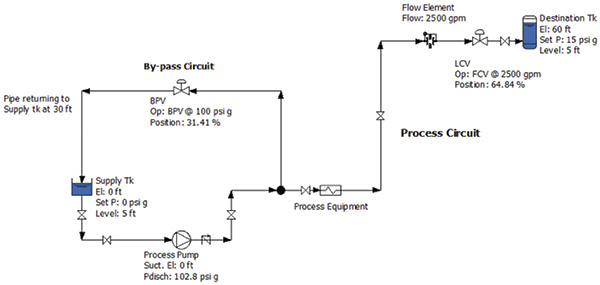 Figure 1. The operating data from installed plant instrumentation and elevations of selected tanks and equipment
Determining Pump Flow Rate
Last month’s column calculated a pump head of 235 feet (ft) and a flow rate of 4,000 gallons per minute (gpm). From the pump curve, it was determined that the pump had an efficiency of 83 percent at its flow rate. The pump’s operating costs were calculated after looking at the pump’s motor efficiency, annual hours of operation and cost of electrical power. So how was the flow rate through the pump of 4,000 gpm established? The flow to the destination tank is 2,500 gpm, but because there is no flow element in the bypass circuit, the pump’s total flow rate cannot be calculated. Without this value, the pump efficiency and power consumed also cannot be calculated. The pump curve is the key to this process because it provides manufacturer-supplied test data on how the pump operates for its flow range. Knowing the pump’s total head, the pump curve can be entered on the head axis and move across until the known pump head value intersects the pump curve. Dropping straight down on the pump curve gives the flow rate, and the intersection point provides the pump efficiency. In Figure 1, the process pump’s discharge pressure is 102.8 pounds per square inch (psig). Centrifugal pump curves use head instead of pressure, so the discharge pressure must be converted to feet of fluid using Equation 1.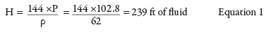
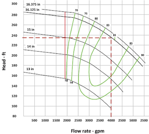 Figure 2. Determining the flow rate and pump efficiency from calculated total head of 235 ft
Static Head Cost
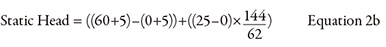
The static head accounts for the difference in fluid energy between the destination and supply tanks. Per the Bernoulli equation, fluid energy is composed of three types of head: elevation, pressure and velocity. Because the fluid is at rest in the supply and destination tanks, the velocity head has no value (see Equation 2).

Process Element Cost
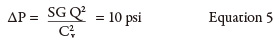
Process equipment—characterized by a head loss that is a function of flow rate—is the next item in the energy cost balance sheet. In the system shown in Figure 1, the process element has no installed pressure gauges. The manufacturer’s equipment data sheet will be used to calculate head loss. The manufacturer’s supplied data sheet could have a curve showing the pressure drop and head loss for a range of flow rates, a Cv value or a single value of pressure drop versus a given flow rate. For this example, the manufacturer provided a 14.4 psi pressure drop with a flow rate of 3,000 gpm. To determine the pressure drop through the process element at 2,500 gpm, the Cv must be calculated using the manufacturer’s supplied data points of 3,000 gpm and 14.4 psi (see Equation 4).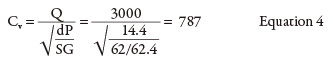

Piping Cost
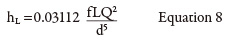
The head loss in a pipeline can be calculated using the Darcy equation (see Equation 7).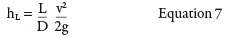
- Reynolds number = 1.23 x 10⁶ unitless
- Relative roughness = 0.00012 in
- Darcy friction factor = 0.0135 unitless
- Pipe head loss = 0.44 ft
- Valve and fitting loss = 0.57 ft
- Pipeline head loss = 1.01 ft
http://kb.eng-software.com/questions/575/Pipeline+Head+Loss+Calculation+Process.) The head losses for the circuit’s remaining pipelines are added to obtain the total pipeline head loss in Table 1.
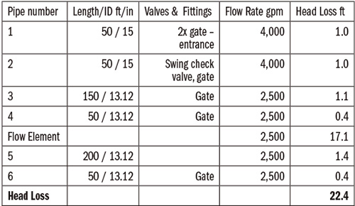 Table 1. Pipeline summary, calculated head loss and annual operating costs for the pipelines in the process circuit
Control Valve Cost
Control valves regulate flow rate to achieve the desired set point—in this case, the level in the destination tank. The tank’s outflow (not shown on the drawing) feeds the plant’s demands. When the flow rates into and out of the tank are equal, the level in the destination tank is constant. To determine the operating cost, the flow rate through and the differential pressure across the level control valve are needed. Most systems do not measure the valve’s differential pressure, which can be calculated knowing the valve position, flow rate and Cv values as a function of valve position. But that requires involved calculations. Instead, the interaction between the pump, process and control elements can be used to calculate the head loss across the control valve. As shown in past articles, all the energy provided by the pump is used by the process and control elements (see Equation 10). hPump = ∑ hProcess + hControl Equation 10a Substituting the calculated value for pump head and the sum of the head loss of the circuit’s process elements, we can determine the head loss across the control valve. 235 = (95 + 23.3 + 22.4) + hControl Equation 10b The annual operating cost of the level control valve is $22,633, after solving for the known flow rate with 94.3 ft of control valve head loss in Equation 11.
