
In the previous article calculating the cost of elements in a piping system (Pumps & Systems, July 2014), the energy consumed and power cost balanced exactly to demonstrate the process. Seldom is life that exact. In the real-world plant, instruments are subject to inaccuracy, pumps may be worn, estimates may be off or the full system may not be accurately represented in the design documents. This month’s article demonstrates how cross-validating the calculated results can ensure the energy cost balance sheet accurately reflects system operation. The key to validating the results is to use multiple means for arriving at the operating cost of each item in the energy cost balance sheet. If the energy cost balance sheet does not add up, troubleshooting skills need to be employed to discover the reason for the difference. This article will continue to use the example piping system presented in previous articles (see Figure 1).
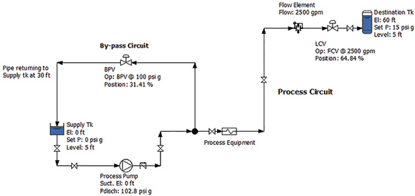 Figure 1. Drawing of sample piping system (Article graphics courtesy of the author.)
Prioritizing the System
The pump elements provide all the energy that enters the system. That energy is then consumed by the system’s process and control elements. If the energy cost balance sheet does not balance, operators should begin looking for the source of the problem. The major energy users in the system should be examined, and operators should find methods to cross-validate the initial estimates.Pump Performance
In the example, the pump’s flow rate was determined using the manufacturer’s pump curve. With a known flow rate, the pump efficiency can be determined from the curve. Because the pump efficiency is used in all energy cost calculations, ensuring the accuracy of the value is critical. Inaccuracies can occur in real-life operating conditions. For example, if the pump has a worn impeller and excessive internal leakage, it no longer reflects the pump curve’s operation. Figure 2 shows a pump curve for the process pump along with an example of the effect that excessive internal leakage can have on the pump curve.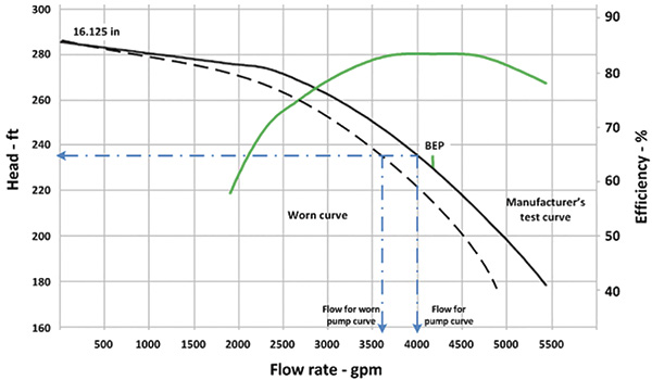 Figure 2. An example showing the effect internal leakage has on pump performance. Because of internal leakage, the installed pump is not operating as designed.
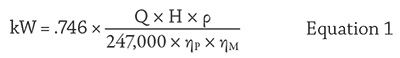 Where:
Q = flow rate in gpm
H = pump head in ft
ρ = fluid density lb/ft3
ηP = pump efficiency
ηM = motor efficiency
If a power reading is not available for the motor, the motor’s power consumption can be calculated by measuring the current and voltage supplied to the pump’s motor, then using Equation 2. The motor’s power factor can be read on its nameplate.
Where:
Q = flow rate in gpm
H = pump head in ft
ρ = fluid density lb/ft3
ηP = pump efficiency
ηM = motor efficiency
If a power reading is not available for the motor, the motor’s power consumption can be calculated by measuring the current and voltage supplied to the pump’s motor, then using Equation 2. The motor’s power factor can be read on its nameplate.
 Where:
P3ϕMotor = motor power in kW
V = voltage volts
I = current amps
Pf = motor power factor
If the calculated value of motor power equals the pump’s power consumption, the pump flow, head and efficiency values are validated.
Where:
P3ϕMotor = motor power in kW
V = voltage volts
I = current amps
Pf = motor power factor
If the calculated value of motor power equals the pump’s power consumption, the pump flow, head and efficiency values are validated.
Tank Levels and Pressures
The tanks and vessels make excellent piping system boundaries. The energy at each tank can be determined by using the elevation of the liquid level in the tank and pressure on the liquid surface. From these values the energy consumed for the static head component can be easily calculated. The results can be cross-validated using installed pressure and level instrumentation. The liquid level can be checked with a sight glass or by manually measuring the liquid level in the tank. The pressure in a closed vessel can be compared using the installed plant instrumentation, installed pressure gauges or a temporary pressure gauge.Control Valves
In last month’s example, the differential pressure across the control valve was calculated by subtracting the sum of the head losses of the process elements from the pump head. This approach is easy, but any errors made in the previous calculations will compound and can greatly reduce the energy cost balance sheet’s accuracy. Valve manufacturers define the operation of control valves based on tests that are outlined in published industry standards. Manufacturers use the ANSI/ISA-75.01.01 Flow Equations for Sizing Control Valves to size control valves for piping systems. The data used in valve sizing can also be used to calculate the differential pressure across the control valve. Equation 3 shows the basic formula for valve sizing.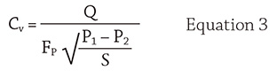 Where:
Cv = manufacturer-supplied valve coefficient
Q = flow rate in gpm
FP = piping geometry factor (unitless)
P1 = absolute pressure measured at valve inlet in lb/in2
P2 = absolute pressure measured at valve outlet in lb/in2
S = fluid specific gravity (unitless)
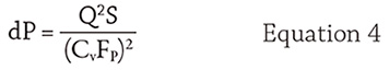
Rearranging the control valve sizing equation and solving for differential pressure results in Equation 4.
Where:
Cv = manufacturer-supplied valve coefficient
Q = flow rate in gpm
FP = piping geometry factor (unitless)
P1 = absolute pressure measured at valve inlet in lb/in2
P2 = absolute pressure measured at valve outlet in lb/in2
S = fluid specific gravity (unitless)
Rearranging the control valve sizing equation and solving for differential pressure results in Equation 4.
 In the example system with a flow rate through the level control valve of 2,500 gpm, the control valve position is 65 percent. According to the manufacturer’s data for the control valve, the Cv at this position is 391.
The FP of .9996 was calculated by the manufacturer and included in the valve data sheet. The specific gravity of the process fluid was calculated at .993. The flow rate through the level control valve was measured at 2,500 gpm. Inserting the values into Equation 4 provides the differential pressure across the control valve.
In the example system with a flow rate through the level control valve of 2,500 gpm, the control valve position is 65 percent. According to the manufacturer’s data for the control valve, the Cv at this position is 391.
The FP of .9996 was calculated by the manufacturer and included in the valve data sheet. The specific gravity of the process fluid was calculated at .993. The flow rate through the level control valve was measured at 2,500 gpm. Inserting the values into Equation 4 provides the differential pressure across the control valve.
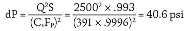 Converting the control valve’s differential pressure of 40.6 pounds per square inch (psi) to feet of fluid results in a head loss of 94.3 ft. This result for the control valve calculation validates the number from last month’s calculations.
